Intro to QGIS Workshop | London Geo Meetup

Overview

This workshop is designed for a beginner-friendly 30 minute walkthrough. It covers getting started with QGIS, loading common geospatial formats, understanding coordinate reference systems, basic styling and labels, filtering, and a small introductory analysis exercise.

Learning Goals

By the end of the workshop, participants should be able to:

• Open QGIS and understand the main parts of the interface.
• Load GeoJSON, Shapefile, and CSV data.
• Check and change layer and project coordinate reference systems.
• Apply simple styles and labels.
• Filter data using the attribute table.
• Run a first analysis workflow using buffers and spatial selection.

What To Prepare Before The Session

1. Install the latest long-term release of QGIS.
2. Download the workshop datasets.

Suggested Datasets

Use one simple dataset for each common format.

It is simpler to use one small OSM-derived central London dataset in three formats so everyone uses the same data during the workshop.

Download the workshop files directly:

• GeoJSON dataset
• CSV dataset
• Shapefile ZIP
• LSOA GeoPackage

GeoJSON

• Use central-london-poi.geojson generated from OSM
• Why this works well: it is small, current OSM data, and easy to inspect, style, label, and filter in QGIS.

Shapefile

• Use the ZIP created from central-london-poi-shp.
• Inside the ZIP, attendees will get the .shp, .shx, .dbf, and .prj files together.
• Why this works well: it demonstrates the multi-file Shapefile structure while keeping the dataset consistent with the GeoJSON and CSV versions.

CSV

• Use central-london-poi.csv generated by ogr2ogr.
• Why this works well: it gives attendees a flat table with coordinates that they can import using Add Delimited Text Layer.

Backup Dataset Options

If one of the primary datasets is inconvenient to download, use one of these alternatives:

• GeoJSON alternative: a local authority or ward boundary GeoJSON from the ONS Open Geography portal.
• Shapefile alternative: Natural Earth rivers, roads, or admin boundaries.
• CSV alternative: a simple spreadsheet with place names and longitude and latitude columns.

Workshop Run Sheet

Follow the steps in order during (or after) the session. Match with the screenshots of what your output was like.

Step 1: Launch QGIS And Save A New Project

1. Open QGIS.
2. Start a new blank project.

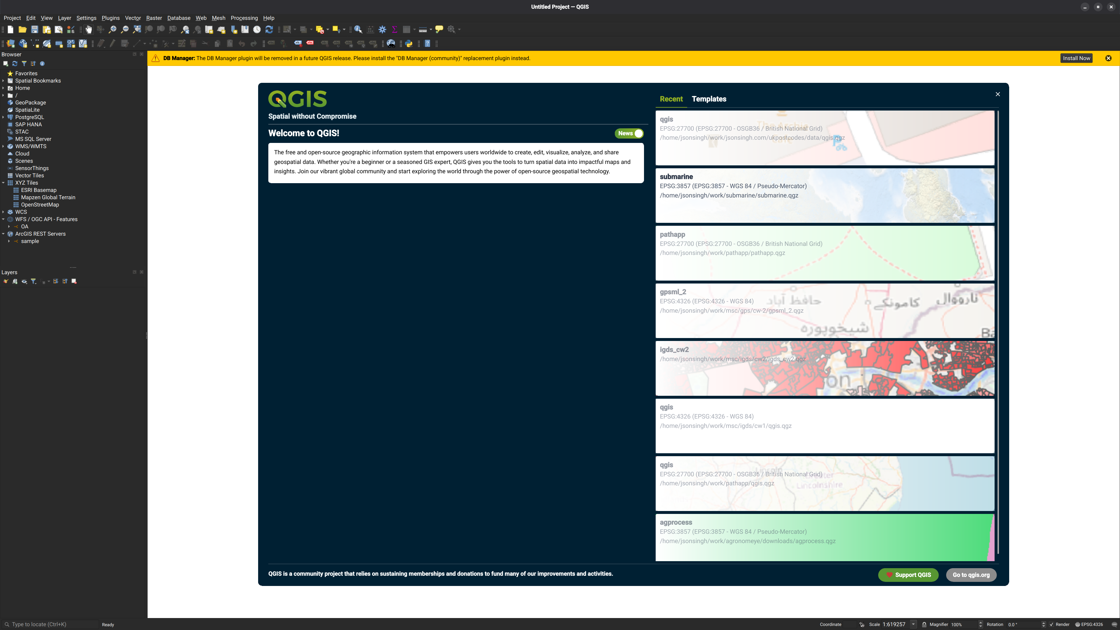
Expected result:

• QGIS is open with an empty map canvas.
• The Browser panel, Layers panel, and status bar are visible.

Step 2: Get Oriented In The Interface

Point out these parts of the application:

• Browser panel
• Layers panel
• Map canvas
• Toolbar
• Status bar
• Coordinate display
• Scale selector

Explain that most beginner workflows involve loading layers, checking their attributes, styling them, and exporting results.

Step 3: Load The GeoJSON Layer

1. Go to Layer > Add Layer > Add Vector Layer.
2. Browse to london-boroughs.geojson.
3. Add the layer to the project.

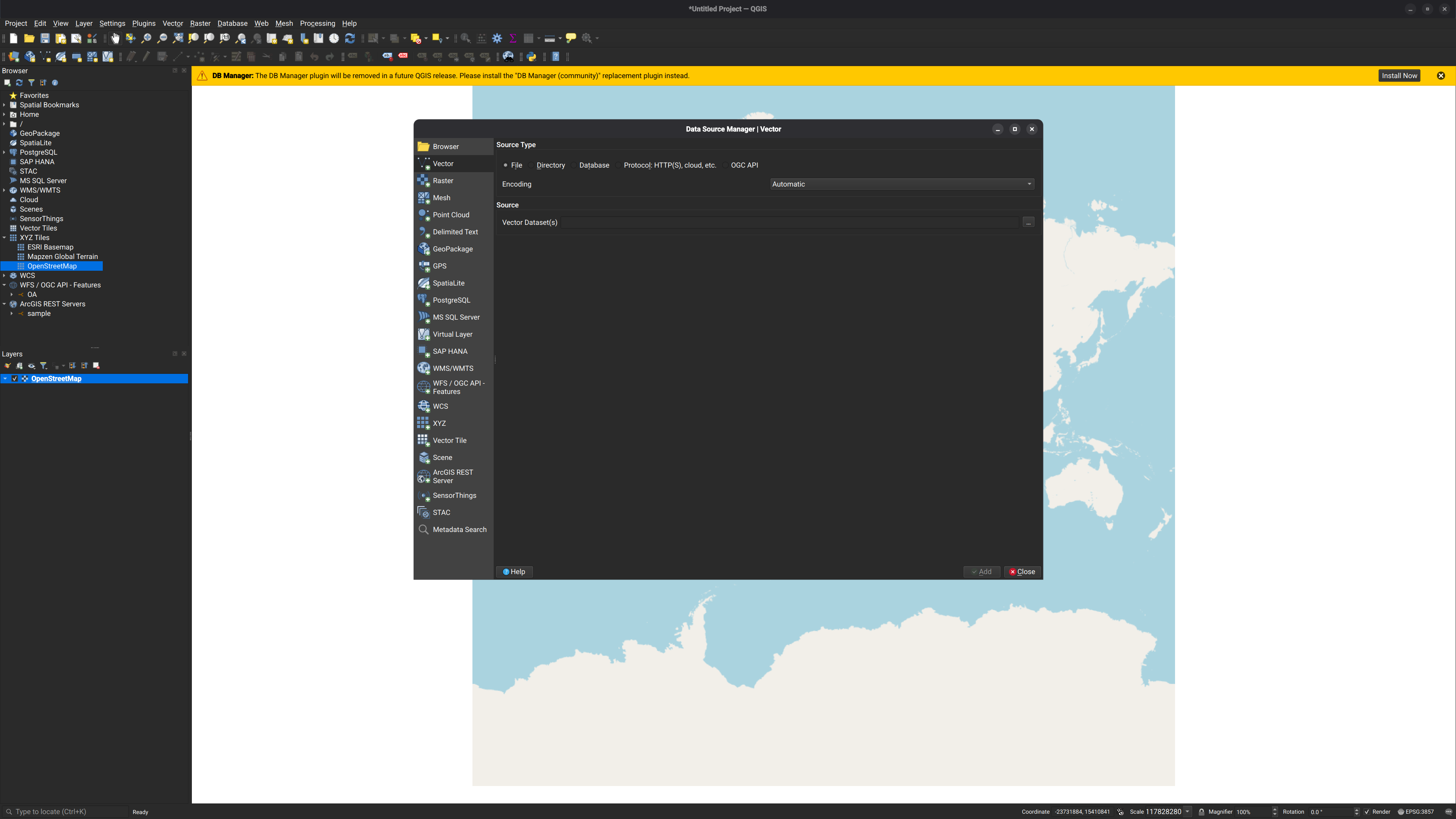
Expected result:

• London borough polygons appear in the map canvas.
• A new polygon layer appears in the Layers panel.

Step 4: Load The Shapefile Layer

1. Extract the Natural Earth ZIP if you have not already.
2. In QGIS, use Add Vector Layer again.
3. Browse to ne_10m_populated_places.shp and add it.

Expected result:

• A second vector layer is added.
• Point features appear, although they may be tiny at first.

Step 5: Load The CSV As A Point Layer

1. Go to Layer > Add Layer > Add Delimited Text Layer.
2. Choose central-london-poi.csv.
3. Set the X field to X.
4. Set the Y field to Y.
5. Set the geometry CRS to EPSG:4326 - WGS 84.
6. Add the layer.

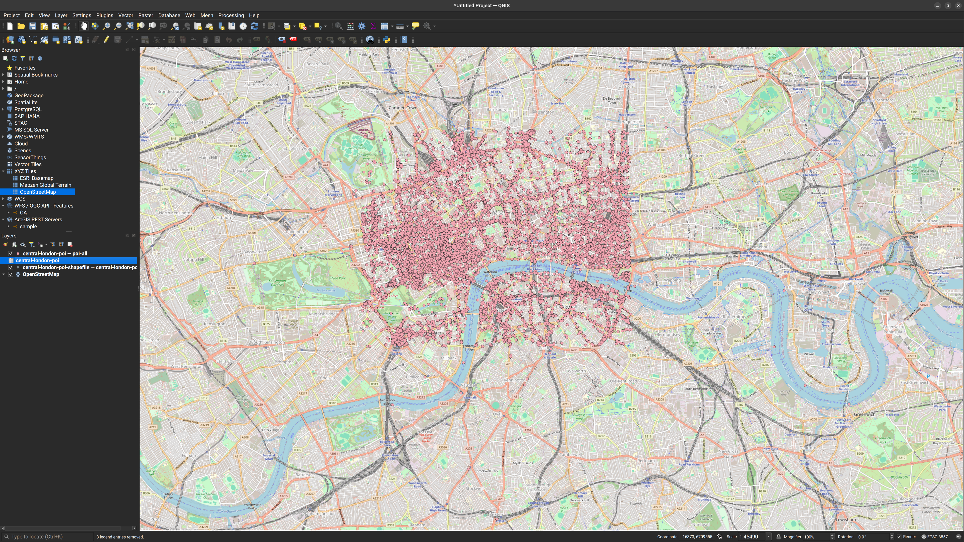
Expected result:

• The CSV is drawn as point features.
• The points should land in London.

Step 6: Inspect Attribute Tables

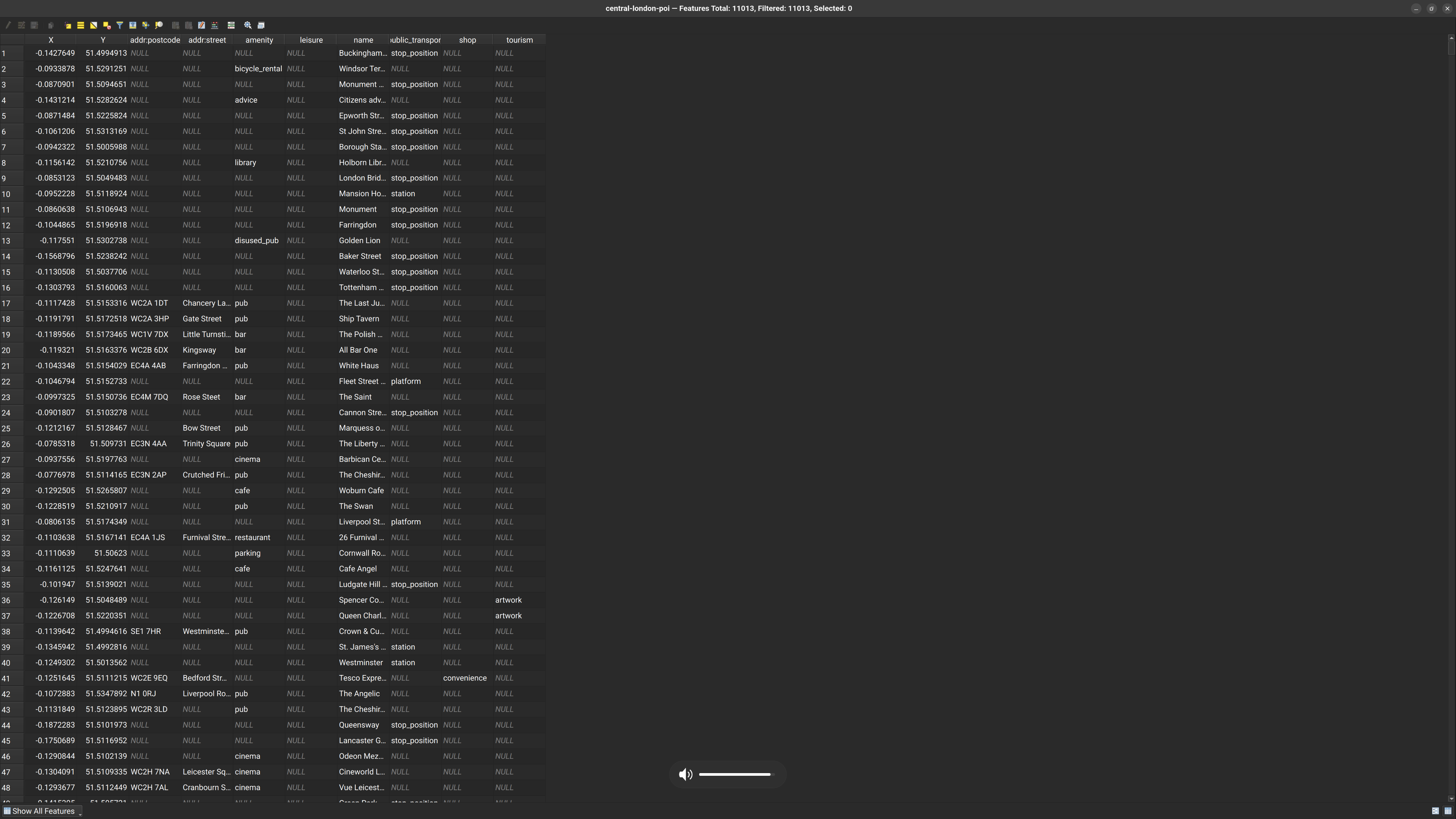
1. Right-click the CSV points layer and open its attribute table.
2. Compare the columns and record structure.

Step 7: Check The Layer CRS And Project CRS

1. Right-click the borough layer and open Properties.
2. Check the layer CRS.
3. Do the same for the CSV layer.
4. Look at the project CRS in the status bar at the bottom of QGIS.

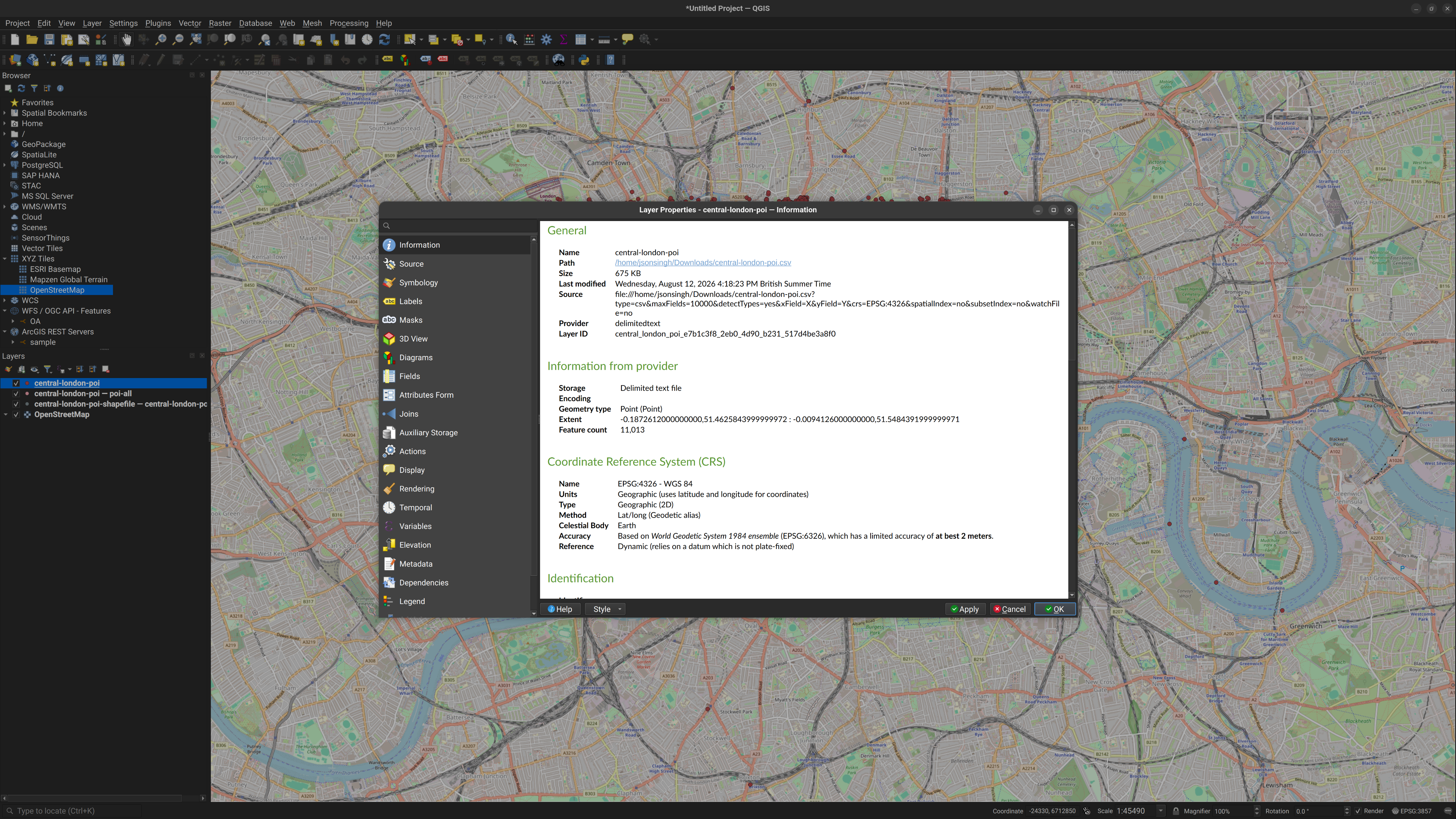
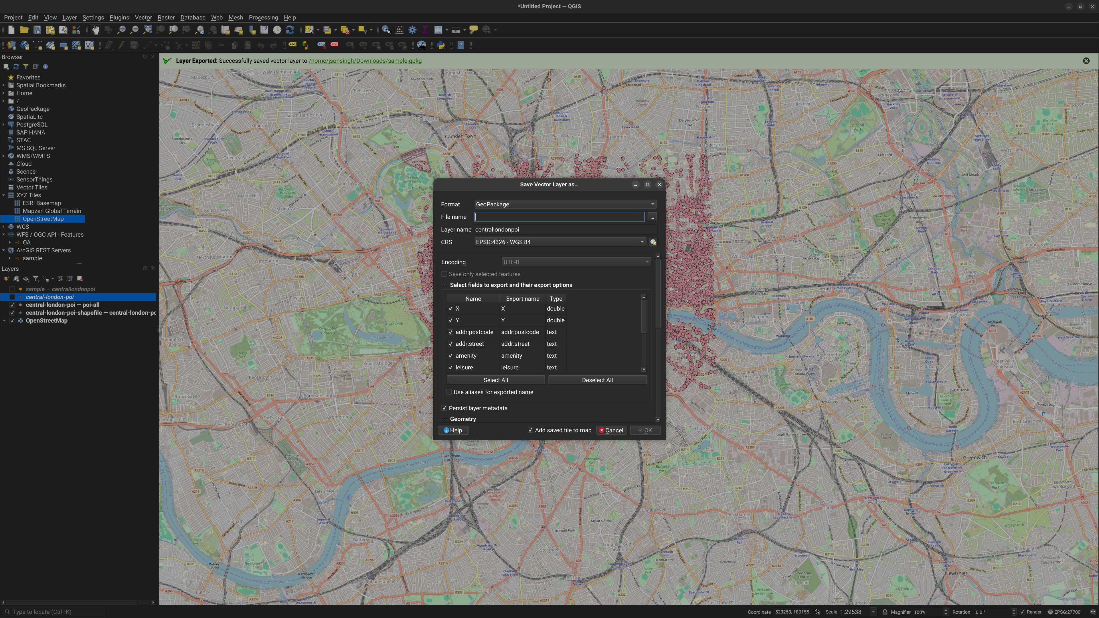
Step 8: Reproject A Layer To British National Grid

1. Right-click the CSV point layer.
2. Choose Export > Save Features As....
3. Set the format to GeoPackage or Shapefile.
4. Set the CRS to EPSG:27700 - OSGB 1936 / British National Grid.
5. Save the output into the output folder as central-london-poi-bng.
6. Add the exported layer back into the project.

Expected result:

• You now have an original WGS 84 point layer and a projected British National Grid version.

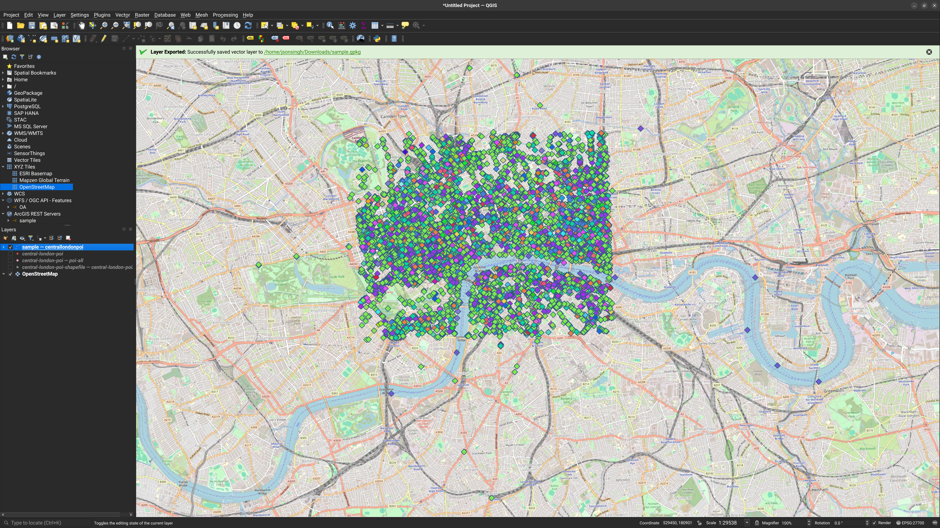
Step 9: Apply Basic Styling

1. Open the borough layer styling panel.
2. Use a simple fill with a light interior and darker outline.
3. Open the central-london-poi.csv or reprojected point layer styling panel.
4. Categorize the points by the amenity field.
5. Apply different colours or symbols for each category.

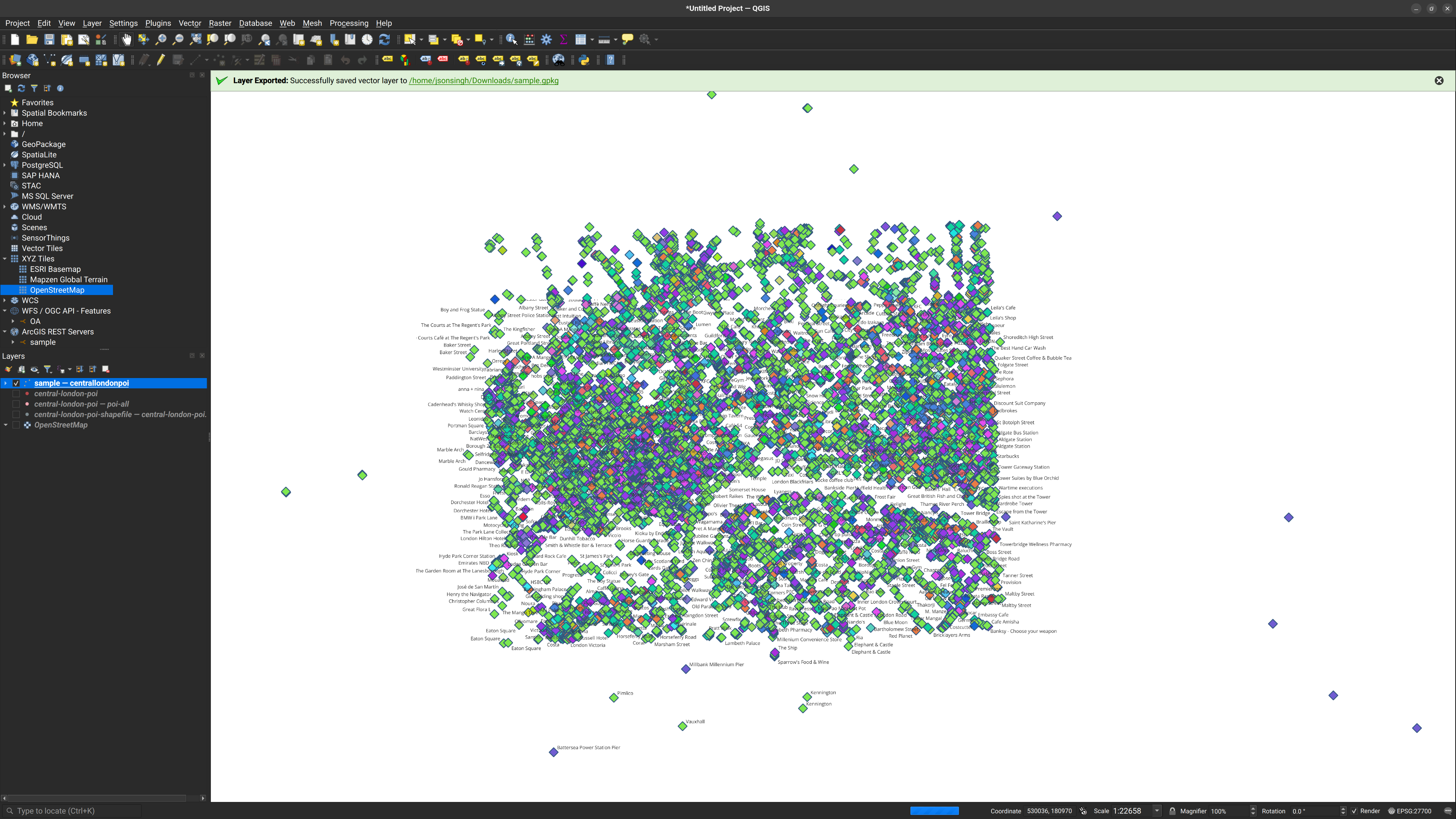
Step 10: Turn On Labels

1. Open layer properties for the CSV points layer.
2. Turn on labels using the name field.
3. Adjust label placement so the names are readable.

Step 11: Filter The Data

1. Open the CSV points layer.
2. Use the filter or query builder.
3. Filter the data to show only amenity = 'cafe' features.
4. Clear the filter afterwards.

Optional borough exercise:

• Filter the borough layer using whichever field contains the borough name.

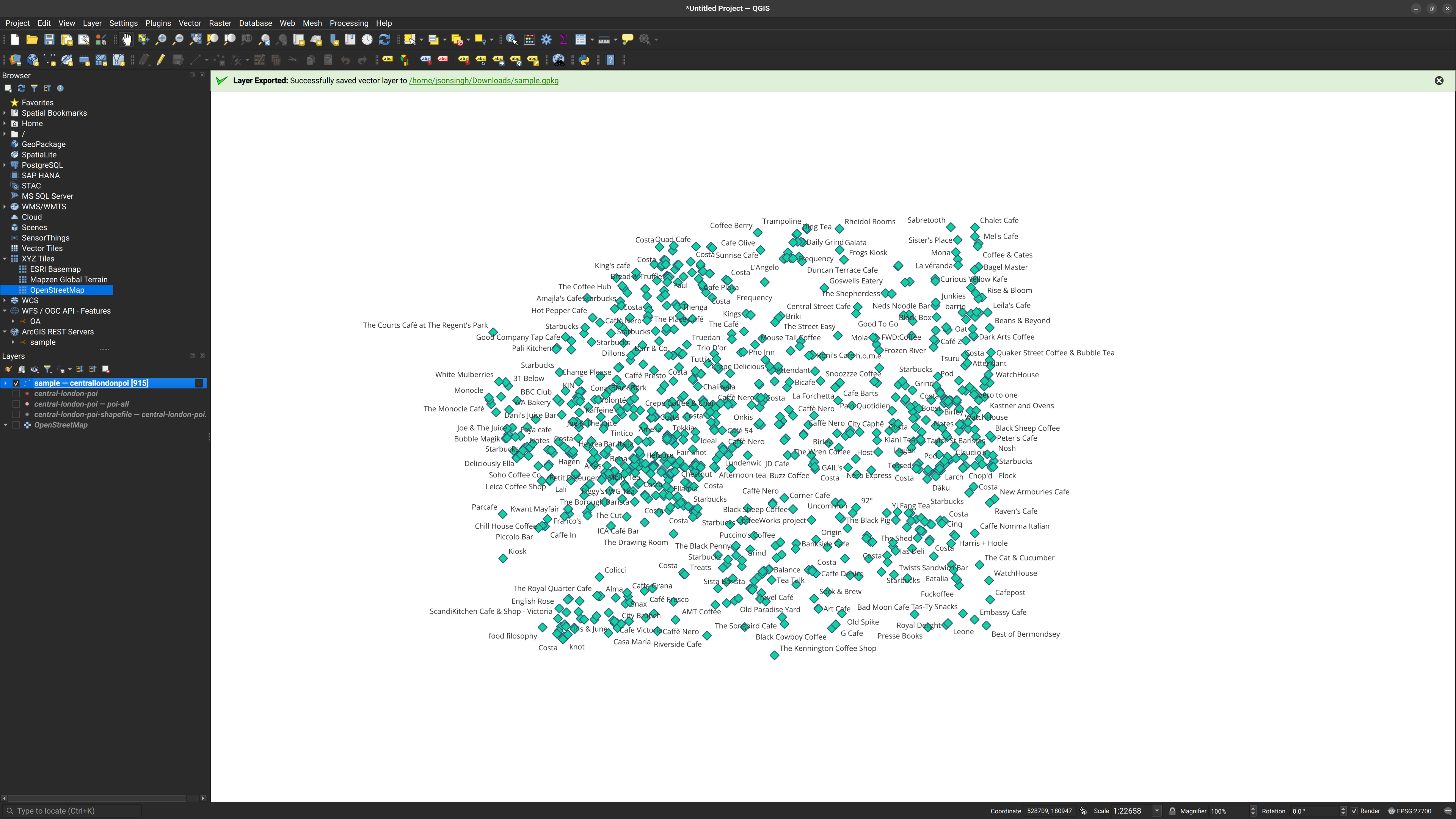
Step 12: Run A Simple Buffer Analysis

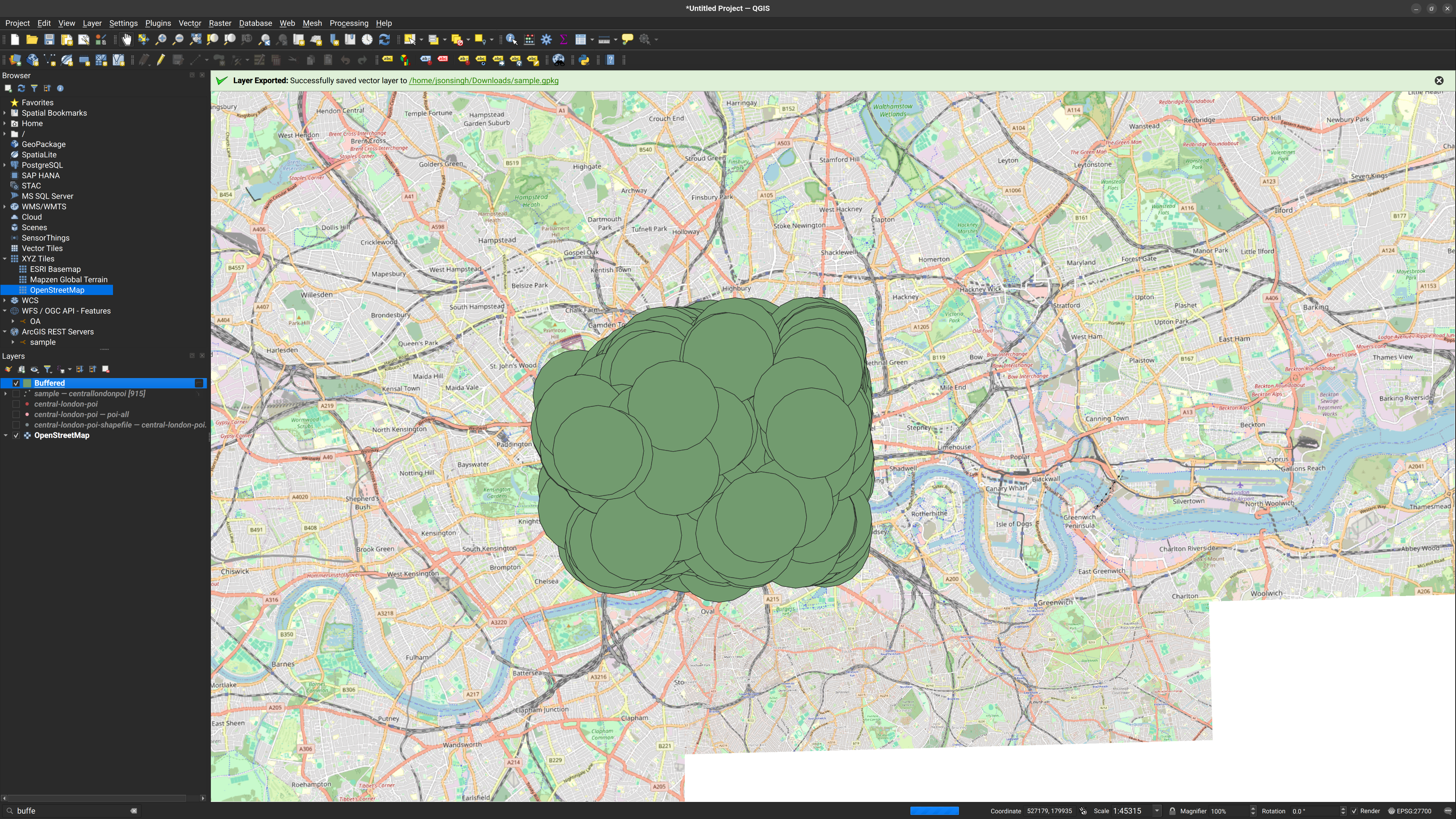
1. Use the reprojected central-london-poi-bng layer for this step.
2. Open the Processing Toolbox.
3. Search for Buffer.
4. Create a 1000 metre buffer around the points.
5. Save the output into the output folder.

Expected result:

• Each point is surrounded by a 1 kilometre polygon buffer.

Step 13: Select Boroughs That Intersect The Buffers

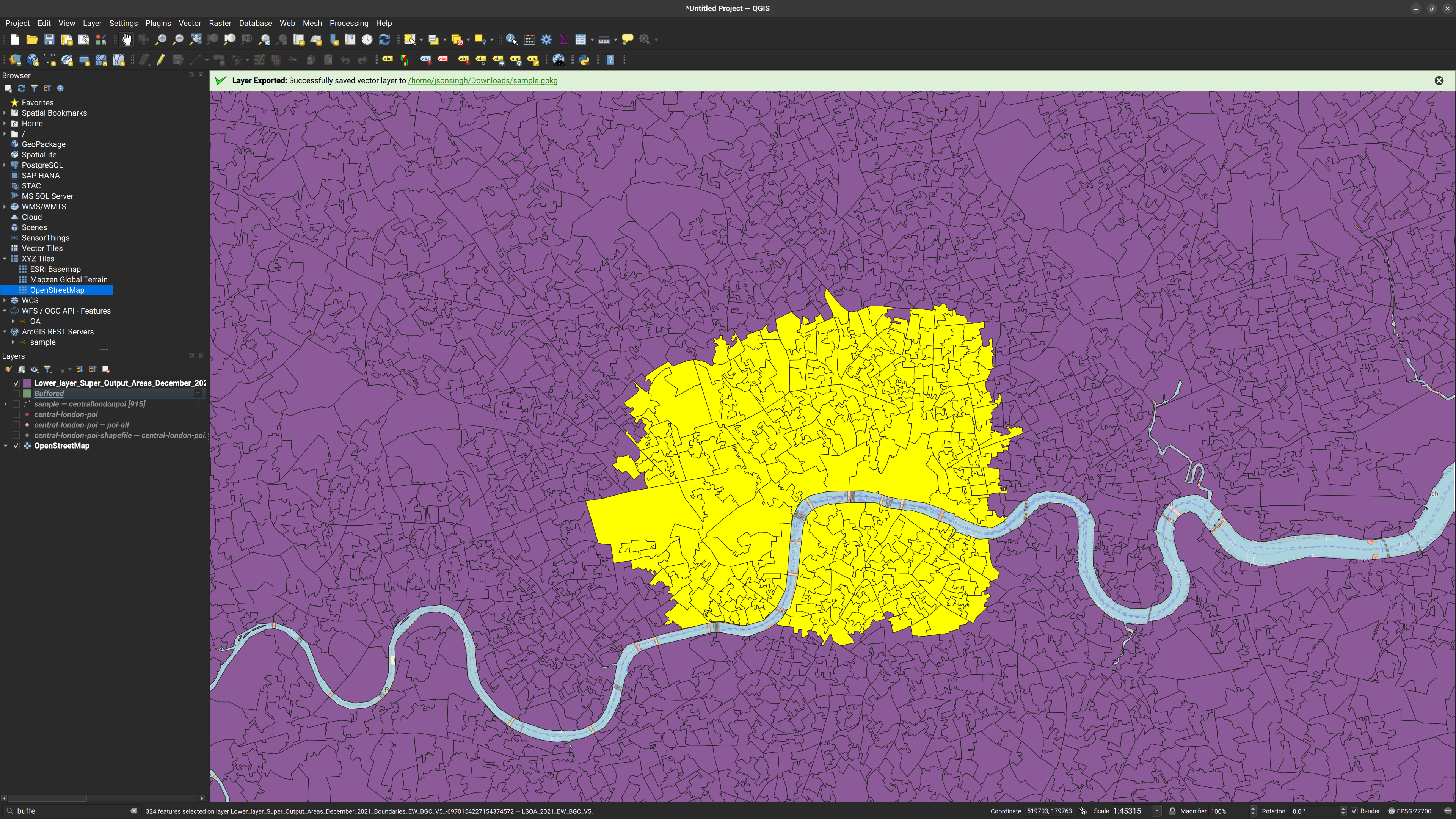
1. Open Vector > Research Tools > Select by Location, or use the Processing Toolbox version.
2. Select features from the borough layer.
3. Use the buffer layer as the intersect layer.
4. Run the tool.

Expected result:

• Boroughs intersecting the buffers become selected.

Step 14: Measure And Discuss What Changed

1. Use the measure tool to check a distance between two visible points.
2. Compare the original point layer and the projected point layer.
3. Ask participants what changed at each stage: loading, CRS, styling, filtering, and analysis.